10. Optimization

# Import some helper functions (please ignore this!)
from utils import * 

Context: We can use NumPyro to perform the MLE on a class of models, composed of discrete distributions. The MLE involves solving an optimization problem—finding the parameters that maximize the joint data likelihood. So far, we’ve let NumPyro take care of this optimization problem for us. But what is NumPyro doing under the hood?

Outline:

• Introduce (exact) analytical optimization, which rely on person to do most of the work via pen-and-paper math.

• Introduce (approximate) numerical optimization, which rely on the machine to do the work for us, like NumPyro.

• Discuss tradeoffs between the two.

10.1. Analytic Solutions to Optimization Problems

Goal: Let \(\mathcal{D}\) represents our entire data, and \(\mathcal{D}_n\) represent our \(n\)th observation. Recall that our goal is to maximize the joint data log-likelihood:

(10.1)\[\begin{align} \theta^\text{MLE} &= \mathrm{argmax}_\theta \log p(\mathcal{D}; \theta), \end{align}\]

where \(\theta\) represents our model parameters. We will remain consistent with the convention of ML literature; we re-write the above problem as a minimization problem of our negative log-likelihood.

(10.2)\[\begin{align} \theta^\text{MLE} &= \mathrm{argmin}_\theta \underbrace{-\log p(\mathcal{D}; \theta)}_{\text{Our loss function, } \mathcal{L}(\theta)} \end{align}\]

We call the \(\mathcal{L}(\theta)\) our “loss function,” since our goal is now to minimize our losses.

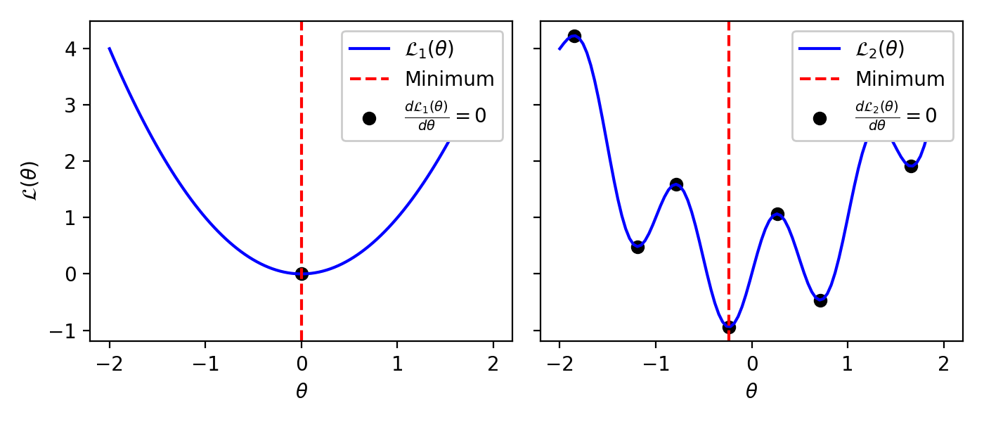
Intuition: So how can we identify the minima of \(\mathcal{L}(\theta)\)? A good place to start is to determine what makes \(\mathcal{L}(\theta)\) different at its minima. Let’s see if we can get some intuition by looking at some intuition by looking at loss functions we made up.

Fig. 10.1 Two “made-up” loss functions—what properties do the minima share?

Looking at the left plot above, we see that the minimum has a unique property: the loss function is flat at the minimum. In other words, at the minimum, the derivative of the loss function equals zero:

(10.3)\[\begin{align} \frac{d \mathcal{L}(\theta)}{d \theta} = 0 \end{align}\]

Does the same hold for the right plot? Not exactly… At the minimum, we do have \(\frac{d \mathcal{L}(\theta)}{d \theta} = 0\). But there are other points for which we also have \(\frac{d \mathcal{L}(\theta)}{d \theta} = 0\). This shows us that there are two types of optima: global and local. The global minima are the \(\theta\)’s that make \(\mathcal{L}(\theta)\) smaller than all other \(\theta\)’s. On the other hand, local minima are \(\theta\)’s that make \(\mathcal{L}(\theta)\) smaller than all other \(\theta\)’s in their neighborhood. Let’s make this clear with the following illustration.

Fig. 10.2 Types of optima. Adapted from this website.

So if our idea of setting the gradient of the loss to zero gives us both global- and local- minima and maxima, is it still useful? Yes, looking at the \(\theta\)’s for which the loss is flat is still helpful! Instead of looking at every possible value of \(\theta\) (in these plots, \(\theta\) can take on infinite different values), we just need to examine the points for which the loss is flat. For the plot on the left, this strategy directly found the global minimum. For the plot on the right, this strategy found a small set of points that includes the global minimum. To find the global minimum within this set, all we need to do is evaluate the loss at each point and select the one that yields the smallest loss.

Procedure: We can turn this intuition into the following four-step process.

1. Compute the derivative of the loss function: \(\frac{d \mathcal{L}(\theta)}{d \theta}\)

2. Set the derivative of the loss function equal to zero: \(\frac{d \mathcal{L}(\theta)}{d \theta} = 0\)

3. Solve the equation for all possible values of \(\theta\) analytically (i.e. on pen-and-paper)—this is the difficult part!

4. Plug each possible value of \(\theta\) into our loss function \(\mathcal{L}(\theta)\) and select the one(s) that minimize it.

10.2. An Example: Analytically Solving for the MLE

The Model. Let’s see how this works by analytically performing the MLE on a simple example. Suppose we want to model the probability of a patient being hospitalized overnight. We can do this using a Bernoulli distribution:

(10.4)\[\begin{align} H \sim p_H(\cdot; \rho) = \mathrm{Bern}(\rho). \end{align}\]

Recall that the PMF of a Bernoulli RV is,

(10.5)\[\begin{align} p_H(h; \rho) = \rho^{\mathbb{I}(h = 1)} \cdot (1 - \rho)^{\mathbb{I}(h = 0)}, \end{align}\]

where \(\mathbb{I}(\cdot)\) is an indicator variable—it evaluates to 1 if the condition in parentheses is true and 0 otherwise.

The Joint Data Likelihood. Now, let’s write the joint data log-likelihood for our model:

(10.6)\[\begin{align} \log p(\mathcal{D}; \rho) &= \log \prod\limits_{n=1}^N p(\mathcal{D}_n; \rho) \quad (\text{since observations are i.i.d}) \\ &= \log \prod\limits_{n=1}^N p_H(h_n; \rho) \\ &= \log \prod\limits_{n=1}^N \rho^{\mathbb{I}(h_n = 1)} \cdot (1 - \rho)^{\mathbb{I}(h_n = 0)} \quad (\text{using the definition of Bernoulli PMF}) \\ &= \sum\limits_{n=1}^N \log \rho^{\mathbb{I}(h_n = 1)} + \log (1 - \rho)^{\mathbb{I}(h_n = 0)} \quad (\text{using the fact that } \log (x \cdot y) = \log x + \log y) \\ &= \sum\limits_{n=1}^N \mathbb{I}(h_n = 1) \cdot \log \rho + \mathbb{I}(h_n = 0) \cdot \log (1 - \rho) \quad (\text{using the fact that } \log x^y = y \cdot \log x) \\ &= \underbrace{\left( \sum\limits_{n=1}^N \mathbb{I}(h_n = 1) \right)}_{\text{Total number of times $H = 1$}} \cdot \log \rho + \underbrace{\left( \sum\limits_{n=1}^N \mathbb{I}(h_n = 0) \right)}_{\text{Total number of times $H = 0$}} \cdot \log (1 - \rho) \quad (\text{moving terms that do not depend on the sums out}) \\ &= T \cdot \log \rho + (N - T) \cdot \log (1 - \rho) \end{align}\]

where \(T = \sum\limits_{n=1}^N \mathbb{I}(h_n = 1)\) is the total number of hospitalizations.

The MLE Objective. Our MLE objective is therefore:

(10.7)\[\begin{align} \rho^\text{MLE} &= \mathrm{argmax}_{\rho} \text{ } \log p(\mathcal{D}; \rho) \\ &= \mathrm{argmax}_{\rho} \left( T \cdot \log \rho + (N - T) \cdot \log (1 - \rho) \right) \\ &= \mathrm{argmin}_{\rho} \underbrace{\left( -T \cdot \log \rho - (N - T) \cdot \log (1 - \rho) \right)}_{\text{Our loss function: } \mathcal{L}(\rho)} \quad (\text{maximizing a function is equivalent to minimizing its negative}) \end{align}\]

Analytic Optimization. We take the gradient of the above loss \(\mathcal{L}(\rho)\) with respect to \(\rho\), set it to \(0\) and solve:

(10.8)\[\begin{align} 0 &= \frac{d \mathcal{L}(\rho)}{d \rho} \\ &= \frac{T - N \cdot \rho}{\rho \cdot (\rho - 1)} \quad (\text{taking the derivative of } \mathcal{L}(\rho)) \\ &= T - N \cdot \rho \quad (\text{multiplying both sides by } \rho \cdot (\rho - 1)) \end{align}\]

Solving the above gives us the solution,

(10.9)\[\begin{align} \rho &= \frac{T}{N}. \end{align}\]

The solution is exactly the proportion of hospitalizations out of the total number of hospital visits!

A Note on Constraint Optimization. Oftentimes, when performing the MLE analytically, we need to constrain the parameters to lie within valid ranges. For example, \(\rho\) should only be allowed to take on values between \(0\) and \(1\). Formally, we express such a constraint as follows:

(10.10)\[\begin{align} \rho^\text{MLE} &= \mathrm{argmax}_{\rho} \text{ } \log p(\mathcal{D}; \rho) \quad \text{subject to} \quad 0 \leq \rho \leq 1 \\ \end{align}\]

In our derivation, it just so happens that the solution already satisfies this constraint. However, for different models, we may have to enforce such constraints explicitly. To enforce these constraints, one can use lagrange multipliers. We will not cover this method in here, but just want to point out that this class of methods exists.

10.3. Challenges with Analytic Solutions to Optimization Problems

As you can see from the above example, performing optimization analytically suffers from two challenges:

1. Analytic optimization needs a specialized solution for every model. As you can see from the above example, performing the optimization analytically will require a new derivation for each model. However, when working with real data, we rarely know what’s the “right” model a priori. We typically start with an exploratory data analysis, try different models, evaluate them using different metrics, make hypotheses for why the models don’t fit well, revise the models to fit better, and repeat. If we had to derive a new solution for every model we wish to test, our modeling process will become quite cumbersome. Moreover, we are more prone to make errors in the derivation and write bugs in our code.

2. Analytic optimization cannot solve for the parameters of every model. Since the above example is for a simple Bernoulli model, an analytic solution to the MLE exists. However, for more complex problems, that may not be the case. In fact, for modern ML models, it is rare for there to exist an analytic solution.

This motivates us to look into alternative optimization methods: numeric optimization.

10.4. Numeric Solutions to Optimization Problems

Numeric optimizations algorithms address both shortcomings of analytic optimization:

1. They can be easily applied to different models without cumbersome derivations. This is because they can be conveniently implemented behind abstractions. Moreover, these abstractions allow us to pair different numeric optimization algorithms with different models without having to write much code. They even make it easy to incorporate constraints over the parameters into the optimization. This helps us write bug-free, error-free optimization code.

2. They can be applied to optimization problems for which there exists no analytic optimization solution. They are also fast and work well in practice, making them extremely popular for complicated modern ML models.

Of course, these numerical algorithms have their own challenges—we’ll look into some challenges they face in a bit. Let us introduce the simplest and most popular numerical optimization algorithm: gradient descent.

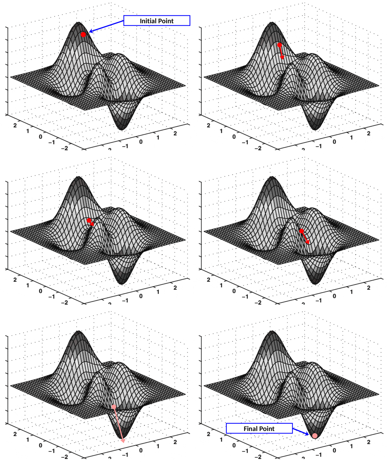
Gradient Descent. The gradient (or “multivariate derivative”) is the direction of the steepest ascent. Similarly, the negative gradient is the direction of the steepest descent. The idea behind the gradient descent algorithm is to take little steps in the direction of the negative gradient in hope that, after taking enough steps, we’ll reach the minimum. Let’s illustrate this with an animation:

Fig. 10.3 Animation of gradient descent on a 2-dimensional function. GIF from this website.

In the animation, the vertical axis represents \(\mathcal{L}(\theta)\). The two horizontal axes represent the dimensions of \(\theta\) (in this case, it’s 2-dimensional). Each arrow represents the negative gradient. As you can see, in each iteration of the algorithm, \(\theta\) (the red point) moves in the direction of the gradient, progressively minimizing the loss.

Now, let’s write the gradient descent algorithm. For clarity, we’ll write it out with the notation for a 1-dimensional \(\theta\) (the multivariate version is pretty much the same).

Algorithm 10.1 (Gradient Descent)

Inputs. A loss function, \(\mathcal{L}(\theta)\), a choice for the learning rate, \(\alpha\), and an initialization for the parameters, \(\theta^\text{current} \leftarrow \text{initial value}\).

Output. Return a parameter \(\theta\) that (hopefully) minimizes the loss \(\mathcal{L}(\theta)\).

Algorithm. Repeat until the loss doesn’t change much from iteration to iteration:

1. Compute the gradient of the loss with respect to the parameters, evaluated at the current value of the parameters:

(10.11)\[\begin{align} u &\leftarrow \frac{d \mathcal{L}(\theta)}{d \theta} \Bigg|_{\theta = \theta^\text{current}} \end{align}\]

2. Take a step in the direction of the negative gradient (steepest descent):

(10.12)\[\begin{align} \theta^\text{next} &\leftarrow \theta^\text{current} - \alpha \cdot u \end{align}\]

3. Update the model parameters:

(10.13)\[\begin{align} \theta^\text{current} &\leftarrow \theta^\text{next} \end{align}\]

In this algorithm, notice that there’s one variable we have yet to define: \(\alpha\). Here, \(\alpha\) represents the size of the step we plan to take in the direction of the gradient. It is typically called the learning rate. You will have to play with this parameter to determine what value works best for minimizing your loss. According to lore, a good place to start is with \(\alpha = 0.01\). Why? Who knows…

Simple Implementation of Gradient Descent. Even though NumPyro already comes with several different gradient-based optimization algorithms, let’s implement the above univariate gradient descent algorithm. While we’re at it, let’s have the algorithm keep track of how our parameters \(\theta\) change with each iteration to get some more intuition:

import jax

def univariate_gradient_descent(loss_fn, num_iterations, learning_rate, theta_init):
    # Initialize theta     
    theta = theta_init

    # For each iteration of the algorithm...
    for i in range(num_iterations):
        # Use Jax to compute the gradient of the loss with respect to theta
        gradient_fn = jax.grad(loss_fn)

        # Evaluate the gradient at the current value of theta
        u = gradient_fn(theta)

        # Take a step in the direction of the gradient
        theta = theta - learning_rate * u

    return theta

Now let’s see if it can successfully find the minimum of a quadratic loss function: \(\mathcal{L}(\theta) = \theta^2\). Since this is a parabola, we know the minimum of this formula should be at \(\theta = 0\). Will our algorithm find it?

# Define our loss function
def quadratic_loss(theta):
    return theta ** 2.0

# Run gradient descent
minimum = univariate_gradient_descent(quadratic_loss, 100, 0.1, jnp.array(-2.0))

# Print out the minimum
print('Minimum at theta =', minimum)

Minimum at theta = -4.0740719526689754e-10

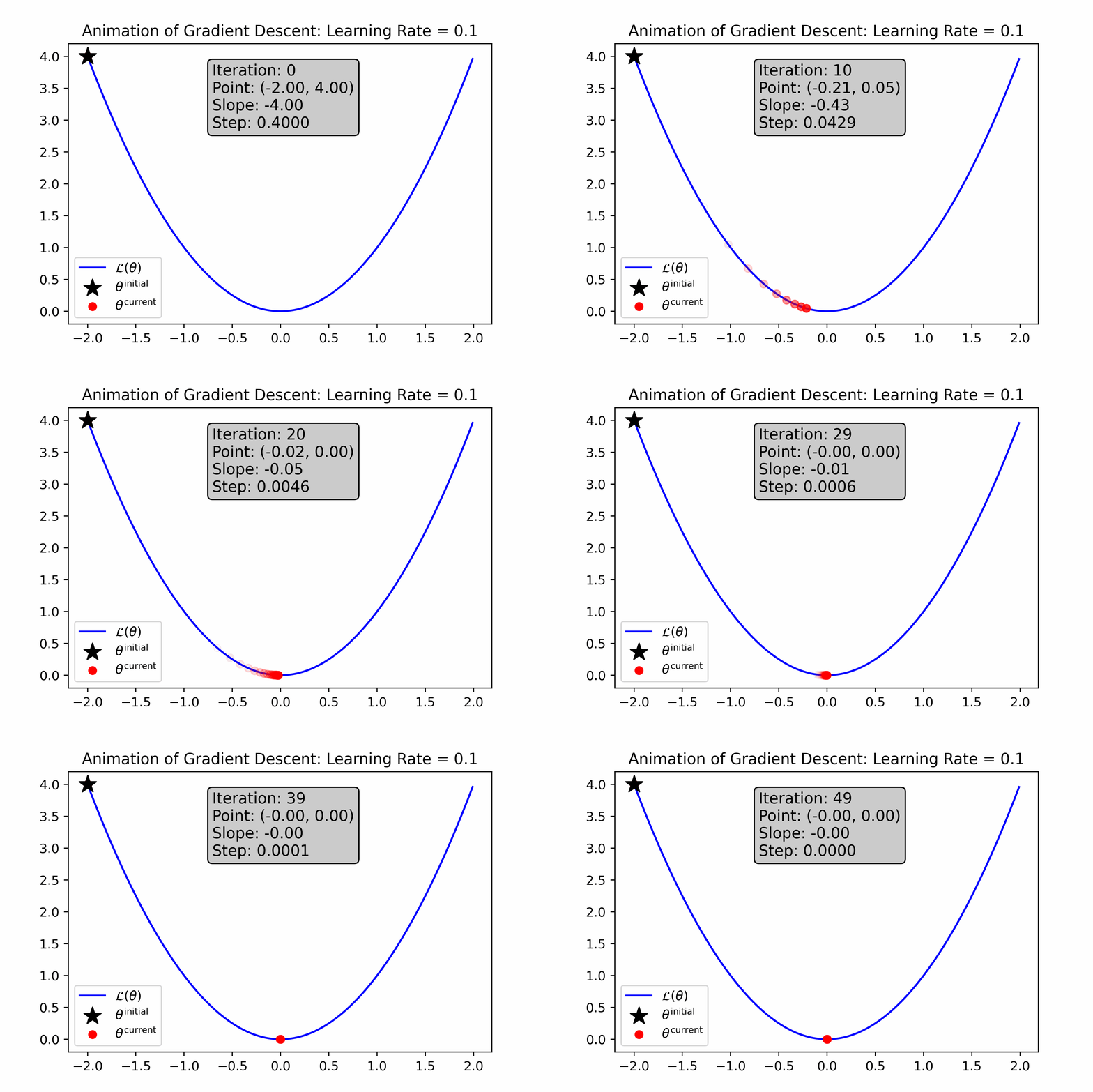
As you can see, gradient descent successfully found the minima, approximately—the resultant number is very close to 0. Let’s animate the algorithm to see how it finds the minima. We’ll do this using two different learning rates: first with \(\alpha = 0.1\), and then with \(\alpha = 0.01\).

Fig. 10.4 For this loss function, a large learning rate causes gradient descent to converge quickly to the minimum.

Fig. 10.5 For this loss function, a small learning rate causes gradient descent to converge more slowly to the minimum.

Exercise: Intuition for Gradient Descent on “Nice” Loss Functions

Look at the two animations above and answer the following questions:

1. Why did a higher learning rate speed up convergence?

2. Notice that gradient descent slowed down with the number of iterations (for both animations). Why does this happen?

Ensuring Parameters Satisfy Constraints. Sometimes we need our parameters to satisfy certain properties. For example, in the above example, in which we computed the MLE for the Bernoulli model, we need to ensure our parameter, \(\rho\), lies on the interval \([0, 1]\). How can we satisfy this constraint using gradient descent? We define \(\rho\) as a function of another variable, \(\psi\), such that the unconstrained \(\psi\) (i.e. \(\psi \in \mathbb{R}\)) is transformed into a constrained \(\rho\) (i.e. \(\rho \in [0, 1]\)):

(10.14)\[\begin{align} \rho &= g(\psi). \end{align}\]

We then perform the optimization over \(\psi\). To make this possible, we need an invertible function \(g(\cdot)\) that maps the real line to the unit interval (i.e. \(g: \mathbb{R} \rightarrow [0, 1]\)). For this, we can use a function known as a sigmoid:

(10.15)\[\begin{align} g(\psi) = \frac{1}{1 + e^{-\psi}}. \end{align}\]

Check out its Wikipedia page to see what it looks like.

Putting this all together, instead of solving our original optimization problem,

(10.16)\[\begin{align} \rho^\text{MLE} &= \mathrm{argmin}_{\rho} \text{ } \mathcal{L}(\rho) \quad \text{subject to} \quad 0 \leq \rho \leq 1, \end{align}\]

we solve,

(10.17)\[\begin{align} \psi^\text{MLE} &= \mathrm{argmin}_{\psi} \text{ } \mathcal{L}(g(\psi)). \end{align}\]

We can then get \(\rho^\text{MLE}\) from \(\psi^\text{MLE}\) by using \(g(\cdot)\):

(10.18)\[\begin{align} \rho^\text{MLE} = g(\psi^\text{MLE}). \end{align}\]

This is how constraints (such as C.unit_interval) in NumPyro are implemented internally. Of course, each constraint relies on a different transform, \(g(\cdot)\).

Automatic Differentiation. So how does NumPyro know to compute gradients automatically for us? The magic is in the function jax.grad, which uses an algorithm called “automatic differentiation” or “backpropagation” to compute exact (not approximate) gradients. We will not get into this topic in the course, but if you’re interested, check out this video to learn more.

10.5. Challenges with Numeric Optimization

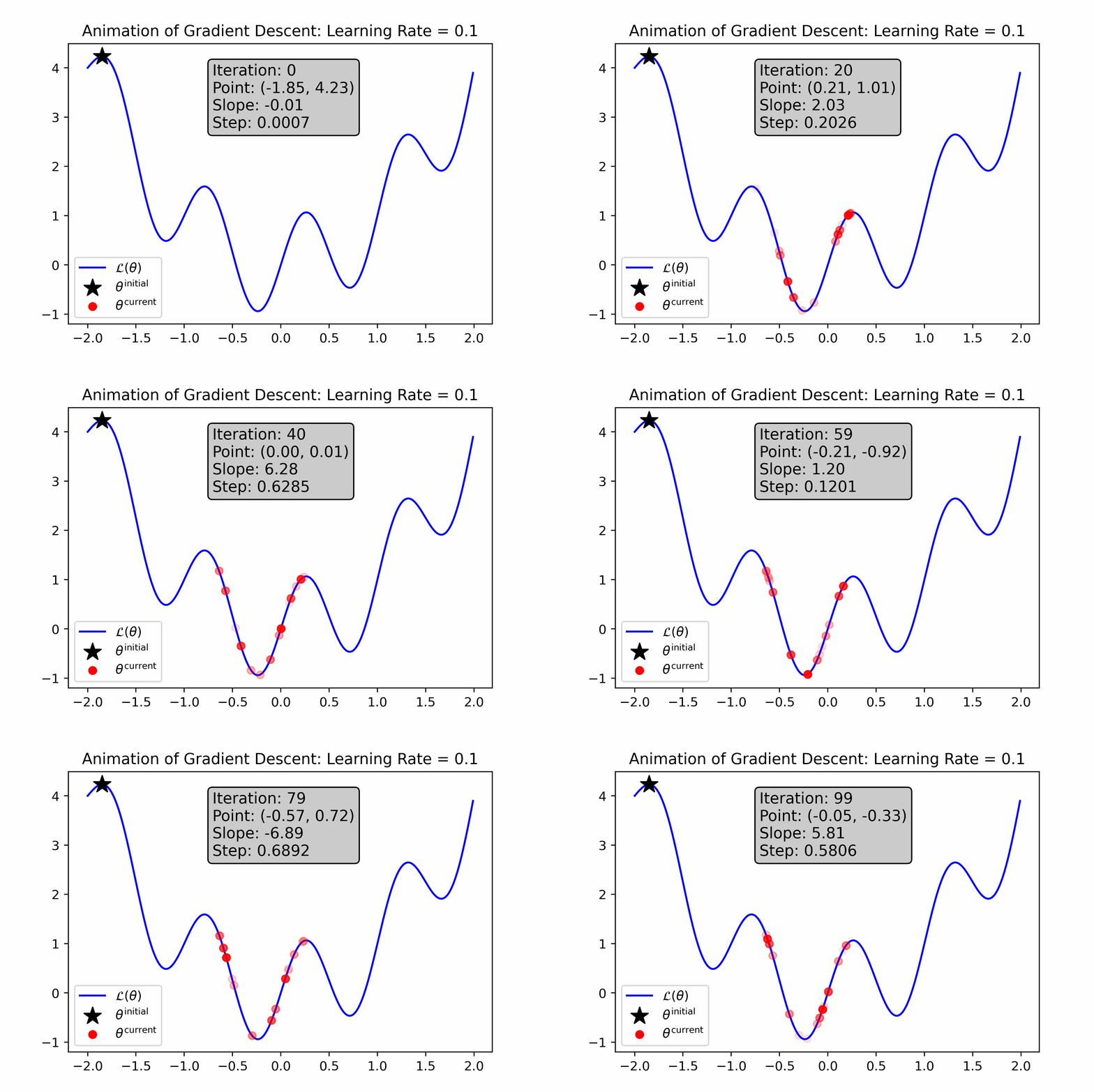
While so far, gradient descent seems like magic, it definitely has its own drawbacks. Let’s look at how gradient descent performs on a more “wiggly” loss function—what do you notice about it?

Fig. 10.6 For this loss function, a small learning rate causes gradient descent to get stuck in a local minimum near its initialization.

Fig. 10.7 For this loss function, a large learning rate helps step out of local minima, but prevents gradient descent from honing in on and ultimately “sticking” to the minimum.

As you can see from these animations, gradient descent struggles with a few challenges:

1. Gradient Descent is Prone to Local Optima. Gradient descent is prone to getting stuck in local optima. Moreover, it’s not possible for us to determine whether an optima is local or global. For some complicated ML models, such local optima can be “good enough” for use, and for others they are not.

2. Gradient Descent is Sensitive to Initialization. Since gradient descent tends to get stuck in local optima that are relatively close to its initialization, it’s important that we try many different initializations to empirically find one that works well. This can be time-consuming.

3. Gradient Descent is Sensitive to Hyper-parameters. As you saw from the above animations, the choice of learning rate and number of iterations change the behavior of gradient descent drastically. This means than whenever we use such numeric optimization algorithm, we will have to try a bunch of different settings of these “hyper-parameters” to empirically see what works best. This can sometimes be time-consuming and cumbersome.

4. Gradient Descent Adds Diagnosic Challenges. Now that we’ve introduced an approximate component to our modeling toolkit—numeric optimization—it will be difficult to diagnose why our ML method performs poorly. For example, if our model fits our data poorly, is it because our modeling assumptions (e.g. our choice of distributions) are inappropriate, or is it because our optimizer got stuck in some local minima?

Given these challenges, it is important for us to use numeric optimization algorithms responsibly: to be aware of all the ways they might fail us, and to think critically about how these failures impact the downstream effects of our ML models.

Exercise: Intuition for Gradient Descent on Non-“Nice” Loss Functions

Part 1: Use this online gradient descent simulator to answer the questions below.

1. Simulate gradient descent for x^2 and then for x^2 + sin(2 * 3.14 * x), each with a starting point of -4 and a learning rate of 0.1. Notice that both functions look similar, but the latter is a “wiggly” version of the former. How do the trajectories differ? Why does this happen?

2. Simulate gradient descent for 1 - exp(-x^2 / 0.1) / 0.1 with a starting point of 2 and a learning rate of 0.1. What is the trajectory like? Why does this happen?

3. Simulate gradient descent for 1 - exp(-x^2 / 0.1) / 0.1 + 0.1 * x^2 with a starting point of 2 and a learning rate of 0.1. What’s the trajectory like? Why does this happen?

Part 2: For each of the situations below, describe what you think the loss function looks like that caused the problematic behavior. Then, describe one way you can mitigate the issue.

1. When training your model, you noticed that initially, your loss function decreased steadily, but after a while, it started bouncing up and down erratically, unable to converge on a minima.

2. When training your model, you noticed your loss function initially decreased steadily, but after a while, it stopped decreasing. You then decide to see how well your model fit your data, and notice that it fits it very poorly.

3. You tried training your model, but the loss didn’t decrease at all.