9. Maximum Likelihood: Code#
# Import some helper functions (please ignore this!)
from utils import *
from cs349 import *
Context: Now that we can describe our objective—to find the model parameters that maximize the probability of the observed data—we are ready to translate it into code.
Challenge: But how can we easily implement this optimization procedure generally? That is, how can we perform the MLE on any model of interest? This is the strength of a probabilistic programming language like NumPyro. Probabilistic programming languages provide us with the necessary abstraction for representing probabilistic models, so that under the hood, NumPyro can help us do the heavy lifting.
Outline:
Use our knowledge of sampling from joint distribution to write down a procedure for sampling from the joint data likelihood.
Directly translate this procedure to
NumPyro.
9.1. The Data Generating Process#
In NumPyro, models are implemented as Python functions. In these functions, we describe the model’s “generative process”—or, a procedure we use to sample the observed data. You just learned how to represent a whole data set using a model (using the plate notation above). We will therefore walk through a specific example that we will then code in NumPyro.
Example: We’ll illustrate how to do this using an example. Suppose we want to model the joint distribution of the day-of-the-week, \(D\), and whether a patient is intoxicated, \(I\). We can do this via the model,
In this model,
Marginal: \(p_D(\cdot; \pi)\) is a distribution over the days of the week. We will therefore define it to be a Categorical distribution:
Conditional: \(p_{I | D}(\cdot | d_n; \rho)\) is the probability that a patient arrives at the ER with intoxication given that \(D = d_n\). Since “intoxication” is a binary outcome, we will model it using a Bernoulli. However, recall that the probability of intoxication changes with the day of the week—on some days, we’re more likely to treat patients with intoxication. The parameter of the Bernoulli distribution therefore needs to change depending on the day of the week. We therefore define:
Valid Parameter Values: Since each entry of \(\rho\) represents a Bernoulli distribution, each entry must be on between 0 and 1 (i.e. on the “unit interval”). And since \(\pi\) represents a Categorical distribution, its entries must sum to 1 (a fancy name of this is that \(\pi\) lies on a “simplex”). We note this briefly because we will have to communicate to NumPyro the valid values these parameters may take on (but don’t worry, this isn’t hard to do).
Generative Process: For this model, we assume the data was sampled (or generated) as follows:
Step 1: We choose an initial guess for \(\pi\) and \(\rho\). Our guess doesn’t need to be good, since
NumPyrohelp us find the right values.Step 2: For every \(n = 1, \dots, N\):
Step 2a: We sample \(d_n\) from the marginal, \(d_n \sim p_D(\cdot; \pi) = \mathrm{Cat}(\pi)\).
Step 2b: Given the specific value of \(d_n\) from Step 2a, we sample from the conditional, \(i_n | d_n \sim p_{I | D}(\cdot | d_n; \rho) = \mathrm{Ber}(\rho_{d_n})\).
This generative process is what we will translate into NumPyro, line for line.
Exercise: Practice with generative processes
Part 1: Write the data generative process for the IHH ER model (described in the exercise in the previous chapter)
Part 2: For each of the DGMs below, write the data-generating process. You can find graphical models for them in the exercise of the previous chapter.
(i) Predictive Models
(ii) Gaussian Mixture Models
(iii) Latent Dirichlet Allocation
(iv) Conditional Subspace Variational Autoencoder
(v) Hidden Markov Models
9.2. Implementing the “Generative Process” (or Model) in NumPyro#
Now that we have our generative process, we can go ahead and implement it in NumPyro. We will do this by relying on three NumPyro primitives. These primitives will communicate to NumPyro everything it needs to know to do the heavy lifting of the MLE. The primitives are:
numpyro.param, which represents model parametersnumpyro.sample, which represents an RVnumpyro.plate, which represents i.i.d sampling using the “plate” notation
We’ll walk you through how to use these primitives to build the model, but we additionally recommend you get in the habit of reading the relevant documentation.
Model: We start by creating a function to represent our model:
def model_of_intoxication_and_day(N, d=None, i=None):
    pass
This function takes in several arguments:
The total number of observations, \(N\).
Optional arrays describing the observations. That is,
drepresents an array of all \(N\) days of the week, andirepresents all \(N\) binary values intoxication-yes/no. When sampling data from the model, we do not pass indandi, but when performing the MLE, we do need to pass them in. This is because the MLE objective will try to find settings of \(\pi, \rho\) that will make our observed data most likely.
Next, we can go through each step of the generative process above and translate it into NumPyro, line by line:
Step 1: We define our parameters using the numpyro.param primitive.
pi = numpyro.param(
    'pi',                          # A name used by NumPyro
    init_value=jnp.ones(7) / 7.0,  # Initial value for pi: [1/7, 1/7, 1/7, 1/7, 1/7, 1/7, 1/7]
    constraint=C.simplex,          # Entries of pi must sum to 1 (i.e. lie on a "simplex")
)

rho = numpyro.param(
    'rho',                         # A name used by NumPyro
    init_value=jnp.ones(7) * 0.5,  # Initial value for rho: [0.5, 0.5, 0.5, 0.5, 0.5. 0.5, 0.5]
    constraint=C.unit_interval,    # Each entry of rho must be in [0, 1] (i.e. lie in "unit interval")
)
You can find more types of constraints listed here.
Step 2: We create a “plate” to indicate \(N\) i.i.d observations using numpyro.plate.
with numpyro.plate('data', N):
    pass
Step 2a: Inside the plate, we sample \(d_n\) from the marginal, \(d_n \sim p_D(\cdot; \pi) = \mathrm{Cat}(\pi)\), using numpyro.sample.
# Define marginal as Categorical using pi
p_D = D.Categorical(pi)

# Sample from the marginal
d = numpyro.sample('d', p_D, obs=d)
Step 2b: Inside the plate, we use the specific value of \(d_n\) from Step 2a to sample from the conditional, \(i_n | d_n \sim p_{I | D}(\cdot | d_n; \rho) = \mathrm{Ber}(\rho_{d_n})\) using numpyro.sample.
# Define conditional as Bernoulli. Notice rho[d] to access the d-th entry of rho
p_I_given_D = D.Bernoulli(rho[d])

# Sample from the conditional
i = numpyro.sample('i', p_I_given_D, obs=i)
Putting everything together: We now have a model that NumPyro understands and can perform MLE on.
import jax
import jax.numpy as jnp
import jax.random as jrandom
import numpyro
import numpyro.distributions as D
import numpyro.distributions.constraints as C


def model_of_intoxication_and_day(N, d=None, i=None):
    pi = numpyro.param(
        'pi',
        init_value=jnp.ones(7) / 7.0,
        constraint=C.simplex,
    )

    rho = numpyro.param(
        'rho',
        init_value=jnp.ones(7) * 0.5,
        constraint=C.unit_interval,
    )

    with numpyro.plate('data', N):
        p_D = D.Categorical(pi)
        d = numpyro.sample('d', p_D, obs=d)

        p_I_given_D = D.Bernoulli(rho[d])
        i = numpyro.sample('i', p_I_given_D, obs=i)
Sampling from the Model: We created a helper function for you, cs349_sample_generative_process, to sample from this model. The function takes in a NumPyro model, a random generator key, and then all arguments your model takes in (in this case, N, d=None, i=None). Note that we haven’t fit the model yet to the data.
N = 20 # Number of samples to generate
key = jrandom.PRNGKey(seed=0) # Random generator key to use

cs349_sample_generative_process(model_of_intoxication_and_day, key, N)
{'pi': Array([0.14285714, 0.14285714, 0.14285714, 0.14285714, 0.14285714,
        0.14285714, 0.14285714], dtype=float64),
 'rho': Array([0.5, 0.5, 0.5, 0.5, 0.5, 0.5, 0.5], dtype=float64),
 'd': Array([1, 1, 0, 2, 5, 3, 3, 0, 1, 5, 5, 3, 4, 2, 0, 1, 1, 3, 6, 4], dtype=int64),
 'i': Array([1, 1, 1, 1, 0, 0, 0, 0, 1, 1, 0, 0, 0, 0, 1, 0, 1, 1, 0, 1], dtype=int64)}
Performing the MLE: We will now perform the MLE using another helper function we’ve created. Recall that the MLE for this model is:
First, we’ll load in the data:
# Import a bunch of libraries we'll be using below
import pandas as pd
import matplotlib.pylab as plt
import numpyro
import numpyro.distributions as D
import jax
import jax.numpy as jnp

# Load the data into a pandas dataframe
csv_fname = 'data/IHH-ER.csv'
data = pd.read_csv(csv_fname, index_col='Patient ID')

# Print a random sample of patients, just to see what's in the data
data.sample(15, random_state=0)
| Day-of-Week | Condition | Hospitalized | Antibiotics | Knots | |
|---|---|---|---|---|---|
| Patient ID | |||||
| 9394 | Friday | Allergic Reaction | No | No | 0 |
| 898 | Sunday | Allergic Reaction | Yes | Yes | 0 |
| 2398 | Saturday | Entangled Antennas | No | No | 3 |
| 5906 | Saturday | Allergic Reaction | No | No | 0 |
| 2343 | Monday | High Fever | Yes | No | 0 |
| 8225 | Thursday | High Fever | Yes | No | 0 |
| 5506 | Tuesday | High Fever | No | No | 0 |
| 6451 | Thursday | Allergic Reaction | No | No | 0 |
| 2670 | Sunday | Intoxication | No | No | 0 |
| 3497 | Tuesday | Allergic Reaction | No | No | 0 |
| 1087 | Monday | High Fever | Yes | No | 0 |
| 1819 | Tuesday | High Fever | Yes | No | 0 |
| 2308 | Tuesday | Allergic Reaction | No | No | 0 |
| 6084 | Monday | High Fever | No | No | 0 |
| 3724 | Tuesday | Allergic Reaction | Yes | Yes | 0 |
Next, we introduce a helper function, cs349_mle, for performing the MLE. This function takes in:
A
NumPyromodel.An optimizer—this is what will do the maximization. We’ll cover optimization at a later chapter. For now, you can just treat them as black boxes.
A random generator key, used by the optimizer.
The number of iterations we’d like the optimizer to run for (this optimization algorithm is iterative).
Finally, we pass in the arguments of the model. In this case, we pass in
N, d=d, i=i. For our modelNis a require argument (for the number of elements innumpyro.plate). You’ll notice that in our model,dandiare both optional. We pass them in here to give the MLE the data (without them, how can we maximize the probability of the data?).
Putting all of this together, we get:
# Get data from the data frame.
# Use our helper function, convert_day_of_week_to_int, to convert the days of the week to ints
d = jnp.array(convert_day_of_week_to_int(data['Day-of-Week']).values)
i = jnp.array((data['Condition'] == 'Intoxication').astype(int).values)

# Number of data points
N = len(d)

# Number of iterations we want the optimizer to take when maximizing the likelihood of the data
NUM_ITERATIONS = 1000

# Pick the size of update to the model's parameter during optimization
LEARNING_RATE = 0.01

# Define an optimizer; here we chose the "Adam" algorithm
optimizer = numpyro.optim.Adam(step_size=LEARNING_RATE)

# Pick a random generator seed for the optimizer
key_optimizer = jrandom.PRNGKey(seed=0)

# Perform MLE!
result = cs349_mle(
    model_of_intoxication_and_day,
    optimizer,
    key_optimizer,
    NUM_ITERATIONS,
    N,
    d=d,
    i=i,
)
0%| | 0/1000 [00:00<?, ?it/s]
0%| | 1/1000 [00:00<08:50, 1.88it/s]
21%|██ | 206/1000 [00:00<00:01, 436.13it/s, init loss: 26390.5733, avg. loss [151-200]: 23682.9217]
41%|████▏ | 413/1000 [00:00<00:00, 815.75it/s, init loss: 26390.5733, avg. loss [351-400]: 23362.6612]
62%|██████▏ | 621/1000 [00:00<00:00, 1130.25it/s, init loss: 26390.5733, avg. loss [551-600]: 23337.1126]
83%|████████▎ | 830/1000 [00:00<00:00, 1382.08it/s, init loss: 26390.5733, avg. loss [751-800]: 23335.6070]
100%|██████████| 1000/1000 [00:01<00:00, 987.60it/s, init loss: 26390.5733, avg. loss [951-1000]: 23335.5544]
Done.
The object returned to us by cs349_mle contains several useful components:
result.model_mleis the fitted model. We’ll need this to sample from the model.result.parameters_mleare the parameters of the fitted model.result.log_likelihoodis the joint data log-likelihood for every iteration of training. This is helpful for visualizing the convergence of the optimizer.
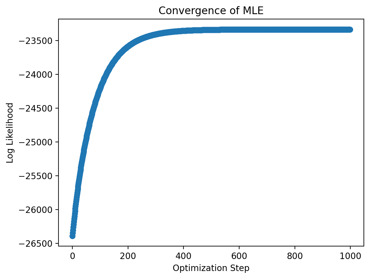
Visualizing the Convergence of the MLE: We can plot the model’s log-likelihood with each iteration of the optimizer to see whether (1) the log-likelihood is increasing, as it should, and (2) whether the optimization converged (i.e. do we think there’s no more room to improve).
plt.scatter(jnp.arange(NUM_ITERATIONS), result.log_likelihood)
plt.xlabel('Optimization Step')
plt.ylabel('Log Likelihood')
plt.title('Convergence of MLE')
plt.show()

Visualizing the Model’s Parameters: The learned model’s parameters, \(\pi\) and \(\rho\), can be accessed as below.
result.parameters_mle
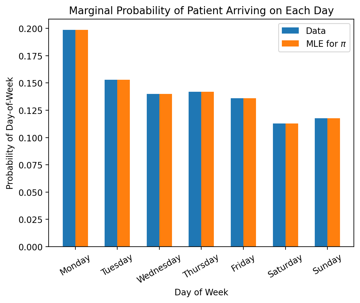
{'pi': Array([0.1987, 0.1529, 0.1399, 0.1419, 0.136 , 0.113 , 0.1176], dtype=float64),
 'rho': Array([0.09473922, 0.09301582, 0.09448023, 0.10785802, 0.10519358,
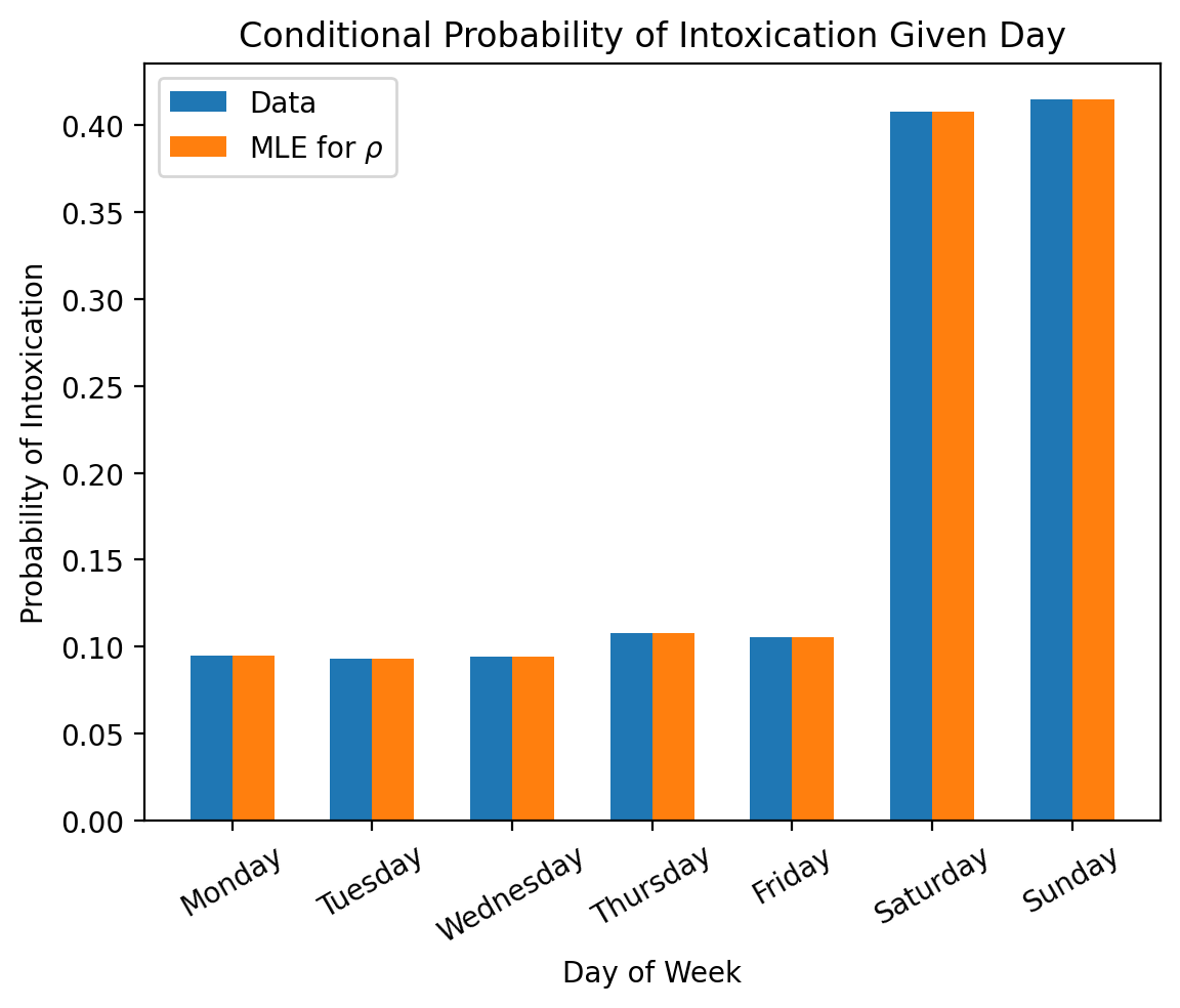
        0.4079646 , 0.41496599], dtype=float64)}
We can then visualize these learned probabilities to see if they match our observed data.
days_of_week = ['Monday', 'Tuesday', 'Wednesday', 'Thursday', 'Friday', 'Saturday', 'Sunday']

marginal_probabilities_from_data = []
conditional_probabilities_from_data = []

# Iterate over the days of the week
for day in days_of_week:
    # Select all patients that came in on the specific day of the week
    patients_on_day = data[(data['Day-of-Week'] == day)]

    # Of the selected patients, further select patients with intoxication
    patient_intoxicated_on_day = patients_on_day[patients_on_day['Condition'] == 'Intoxication']

    # Compute the portion of patients with intoxication on this day
    portion_intoxicated_on_day = float(len(patient_intoxicated_on_day)) / float(len(patients_on_day))

    # Compute the portion of patients arriving on this day
    portion_arriving_on_day = float(len(patients_on_day)) / float(len(data))

    marginal_probabilities_from_data.append(portion_arriving_on_day)
    conditional_probabilities_from_data.append(portion_intoxicated_on_day)
# Plot marginal
width = 0.3
plt.bar(jnp.arange(7) - 0.5 * width, marginal_probabilities_from_data, width, label='Data')
plt.bar(jnp.arange(7) + 0.5 * width, result.parameters_mle['pi'], width, label=r'MLE for $\pi$')

# Add axis labels and titles
plt.xticks(jnp.arange(7), days_of_week, rotation=30)
plt.xlabel('Day of Week')
plt.ylabel('Probability of Day-of-Week')
plt.title('Marginal Probability of Patient Arriving on Each Day')
plt.legend()
plt.show()

# Plot conditional
width = 0.3
plt.bar(jnp.arange(7) - 0.5 * width, conditional_probabilities_from_data, width, label='Data')
plt.bar(jnp.arange(7) + 0.5 * width, result.parameters_mle['rho'], width, label=r'MLE for $\rho$')

# Add axis labels and titles
plt.xticks(jnp.arange(7), days_of_week, rotation=30)
plt.xlabel('Day of Week')
plt.ylabel('Probability of Intoxication')
plt.title('Conditional Probability of Intoxication Given Day')
plt.legend()
plt.show()

Sampling from the Fitted Model: We can sample from the fitted model as follows:
N = 20 # Number of samples to generate
key = jrandom.PRNGKey(seed=0) # Random generator key to use

cs349_sample_generative_process(result.model_mle, key, N)
{'pi': Array([0.1987, 0.1529, 0.1399, 0.1419, 0.136 , 0.113 , 0.1176], dtype=float64),
 'rho': Array([0.09473922, 0.09301582, 0.09448023, 0.10785802, 0.10519358,
        0.4079646 , 0.41496599], dtype=float64),
 'd': Array([1, 1, 0, 1, 4, 3, 2, 0, 1, 5, 5, 3, 4, 2, 0, 0, 1, 3, 6, 4], dtype=int64),
 'i': Array([0, 0, 0, 0, 0, 0, 0, 0, 0, 1, 0, 0, 0, 0, 0, 0, 0, 0, 0, 0], dtype=int64)}
Exercise: Perform the MLE on the IHH ER model
Part 1: You now have all of the tools necessary (1) write the data generating process for the IHH ER model in NumPyro, and (2) perform the MLE on the NumPyro model. We recommend working on parts (1) and (2) together, incrementally building the model. Specifically, we recommend adding distributions in the following order:
a. \(p_D\)
b. \(p_{C | D}\)
c. \(p_{K | C}\)
d. \(p_{H | C}\)
e. \(p_{A | C, H}\)
Please use the following function signature for your model:
def model_of_ihh_er(N, d=None, c=None, k=None, h=None, a=None):
    pass
Part 2: Compare the parameters of each distribution (marginal and conditional) in the learned model with the distributions observed in the data (just like we did above). Do they match?
Part 3: Notice that so far, we’ve relied on a fairly large data-set. But what how good is our learned model if we have a much smaller data set, as is common in many healthcare scenarios? To test this, you can fit your model to a subsample of the data and compare the learned parameters with the distributions observed in the non-subsampled data. That is:
a. We pretend we only observe a small subsample of the data: subsample = data.sample(50, random_state=0).
b. We fit the model to subsample.
c. We then compare the parameters of the learned model to those observed in data.
d. Compare your results to those from Part (2). What do you notice?
